The calculation of the distribution can be a little time-consuming. In the example that appears in the prints of this help, it took around 8 minutes to calculate, being reduced total time in 6498 loopings of the Stepping Stone algorithm.
It may seem fast, but if you lack sufficient CBR material for the final layer for example? In this case, even if the algorithm balances the offers and demands, the result will be flawed because there will be movements with DMT marked as BigNumber.
This happens precisely because there is a lack of good material, or a lack of receive all the bad stuff from the stretch.
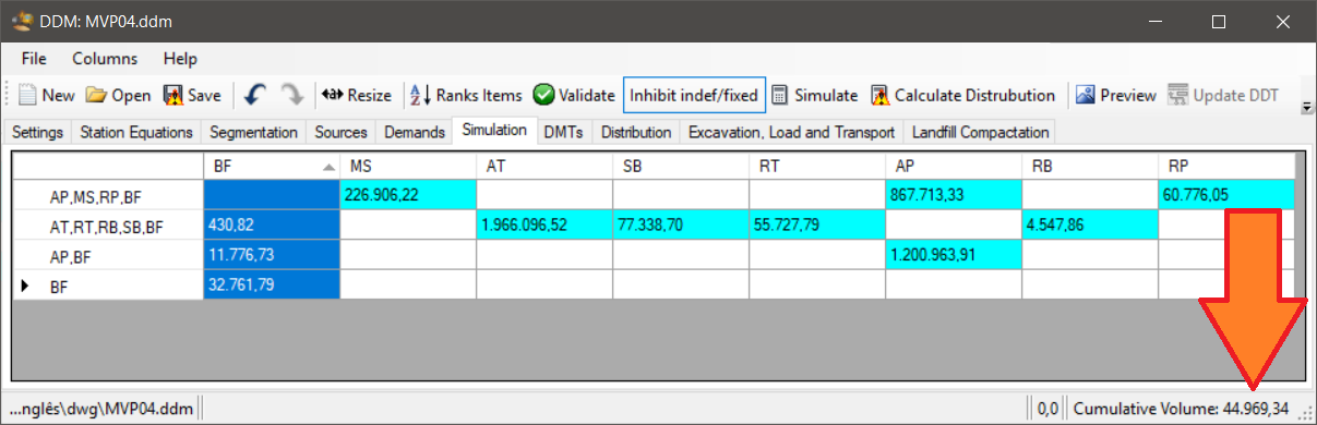
One way to predict this is by simulating the absolute volumes of the origins by track and destinations. So we have a table like this:
Note In the first column, the material ranges and values appear in the first line, the possible destinations.
The values appear in blue because it was possible to allocate in each destination the value total needed.
Note that the distribution is illustrative only. If red cells appear, means that material with adequate CBR, Expansion and Permeability is one or more destinations.
If we select a column, we can see the volume accumulated in the lower corner right, as shown in the figure above.